Raspberry Pi opens a lot of possibilities for do-it-yourself projects. It’s affordable and full of potential for implementing challenging projects. After having spent several years tinkering around my 3D printer, wanting to build my own 3D scanner to complete the 3D workflow was an exciting idea. Using MATLAB and the Raspberry Pi hardware support package for development made the experiment quick and easy, at least from the software perspective.
In this project, I decided to use one of the most basic scanning techniques – focusing more on getting the entire mechanism to work with off-the-shelf components rather than get the best possible results. Raspberry Pi serves as the main controller board for the setup, capturing the images using the Pi Camera, controlling the Line LASER diode and providing control signals to the EasyDriver (Stepper Motor Driver). I have used MATLAB and the Raspberry Pi Hardware support package to implement the algorithm and deploy it to the Raspberry Pi. This step helped me reduce the time required to setup the controller board, and allowed me to focus on getting the mathematics behind the scanning algorithm correct.
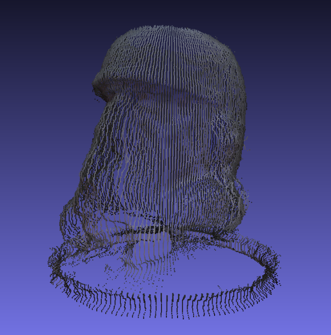
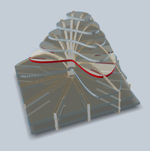
Figure 1: 3D Point Cloud generated using the scanner
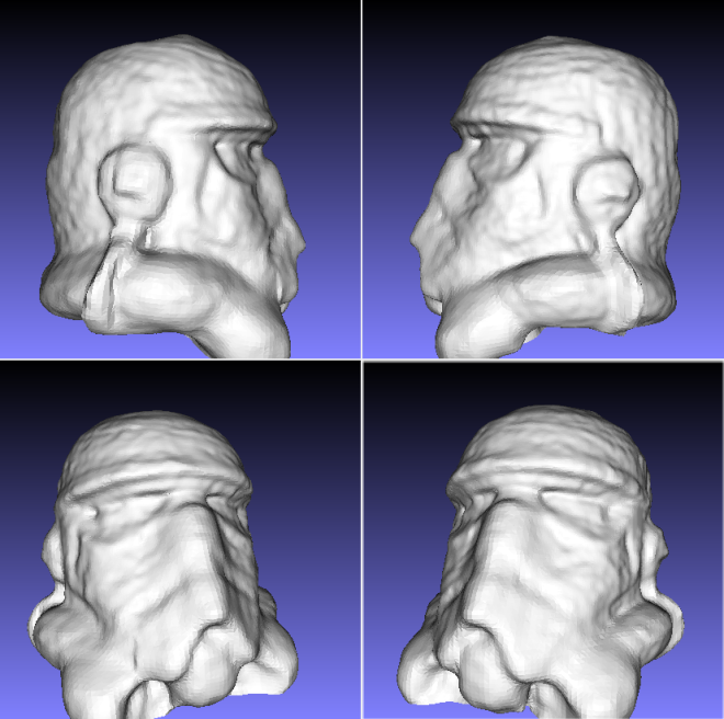
Figure 2: 3D Point Cloud converted into a mesh object using MeshLab and NetFabb Basic
Basic Theory
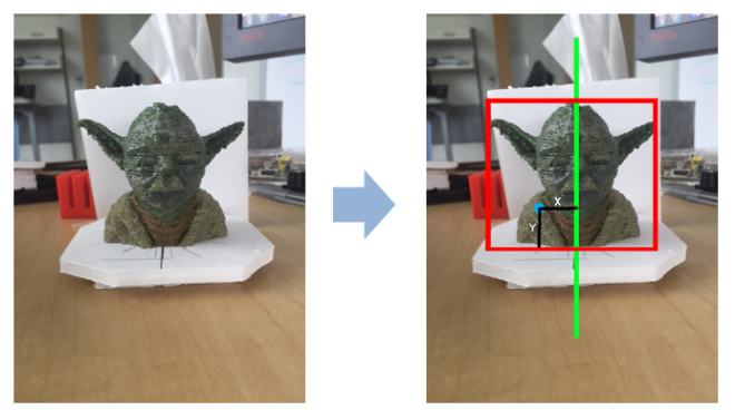
Figure 2: Image of a 3D object
An image of a 3D object provides the projection of the object onto a two dimensional plane. It is trivial to extract the X and Y coordinates of any point on the object since they lie within the image plane. However, the information related to the depth of the point with respect to the center of the object is lost due to the projection. In order to retrieve this information, we need some special help. Thankfully, this is not as difficult as it sounds.
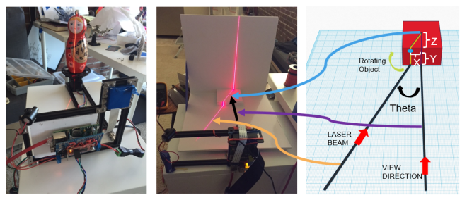
Figure 4: A simple triangulation setup consisting of a Line LASER diode projecting a line on the 3D object
The image above shows a very simple triangulation setup using a camera and a line LASER. The LASER diode is positioned such that it creates a triangle with the view direction of the camera. As you can see from the image, the LASER line projects on the object and intersects the view direction of the camera exactly at the axis of rotation of the object. The angle at the intersection of the LASER line and the view direction (we will call it THETA) provides us with the first tool for extracting depth related information from the image captured by the camera.
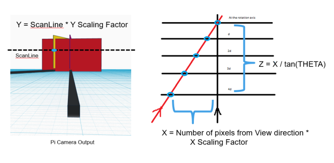
Figure 5: Z-coordinate can be determined by simple trigonometric calculations
Let us assume that the Y coordinate corresponds to each line of pixels in the image and maps to the actual Y coordinate through some scaling factor. At each Y coordinate, the point on the surface of the object where the LASER line projects itself, the intersection of the LASER line with the view direction of the camera (if there was no object to block its path) and the perpendicular dropped from the point on the surface to the view direction form a right-angled triangle. The length of the perpendicular dropped on the view direction gives us the distance of the surface point from the view direction and can be considered as our X coordinate with some scaling factor. The other smaller side of the triangle gives us the depth of the surface point with respect to the axis of rotation, again with a scaling factor. As you can see, the calculations are basic trigonometrical operations.
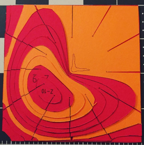
Now, let use this information to build our basic scanning algorithm. In order to extract 3D information of each point lying on the surface of the object, we need to first determine the points at which we can extract this information. This can be achieved very easily by capturing two images – once without the LASER on and once with the LASER on. Since everything else in the view of the camera remains the same, difference of the two images should give us all the points that lie on the LASER line projected on the object. By converting the difference image into a binary image, we can remove most of the extraneous information in the difference image and mark all points lying on the LASER line in white and the remaining pixels of the image as black. We can further narrow down our region of interest by making assumptions about the rectangular area that covers the entire object in the image.
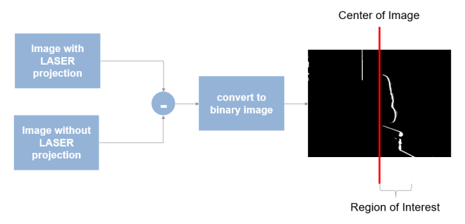
Figure 6: Taking difference of two images of the object – one with the LASER line projected and one without, helps us extract the points that are projected onto the object.
Now we have all the necessary components available for extracting the 3D coordinates of every point lying on the surface of the object. There is still one part that still needs to be taken care of. The points extracted from the images lie on the same image plane and are not oriented correctly in the 3D space. For this, we need to rotated each extracted 3D point by some amount about the axis of rotation. By carefully keeping track of the rotation of the object, we can easily determine the angle by which the points need to be rotated after each rotation step. The final algorithm looks something as shown in the image below.
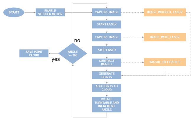
Figure 7: Complete flowchart for steps required to scan a complete 3D object
Prerequisites
For this project, you will need the following hardware and software tools:
- Software:
- MATLAB 2015b+ and Hardware Support package for Raspberry Pi
- Image Processing Toolbox
- Camera Calibration Toolbox
- Point Cloud Toolbox
- MeshLab (tool for generating meshes from point clouds)
- Hardware:
- Raspberry Pi
- Pi Camera
- Line LASER diode
- EasyDriver Stepper Motor driver module
- Stepper Motor
- Optional
- Raspberry Pi prototyping plate
- 3D Printed parts for the turn-table
- MakerBeam kit for the chassis
- Soldering Iron
- Ethernet Cable for connecting the Raspberry Pi to the laptop
- Power Supply – 5v 4A at least
Downloadable Code and Models
You can download the code from:
http://www.mathworks.com/matlabcentral/fileexchange/56861-raspberrypi-+-matlab-based-3d-scanner
You can download the printable parts from:
http://www.thingiverse.com/thing:1622779
Tasks
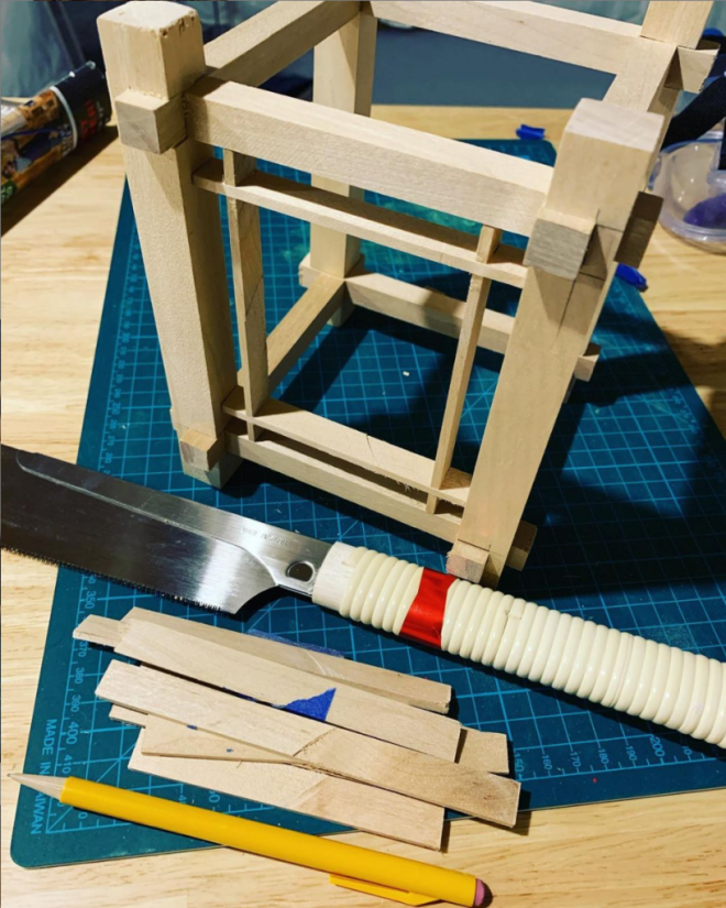
Task 1: Preparing the Chassis
I have used the MakerBeam starter kit to build my chassis for the project. It is easy to use and provides a sturdy base for the camera, LASER diode and the turntable.
You will need the following in order to complete the chassis:
- Two 300mm beams
- Two 200mm beams
- Three 100mm beams
- Two 60mm beams
- 90-degree brackets
- 60-degree bracket for the LASER diode
Use the 60-degree bracket to angle the LASER diode towards the center of the stepper motor placed between the 300mm beams at the other end. Once you connect the camera, you will have to ensure that the center of the stepper motor exactly coincides with the center of the image captured by the camera. With this, the triangulation setup will be complete.
The turn-table can be printed using the models linked in the download section. The base can be fitted directly on top of the stepper motor. The bearing slides into the base and the turntable plate should fall into place on top of the bearing and connecting the shaft coupling connected to the stepper motor shaft.
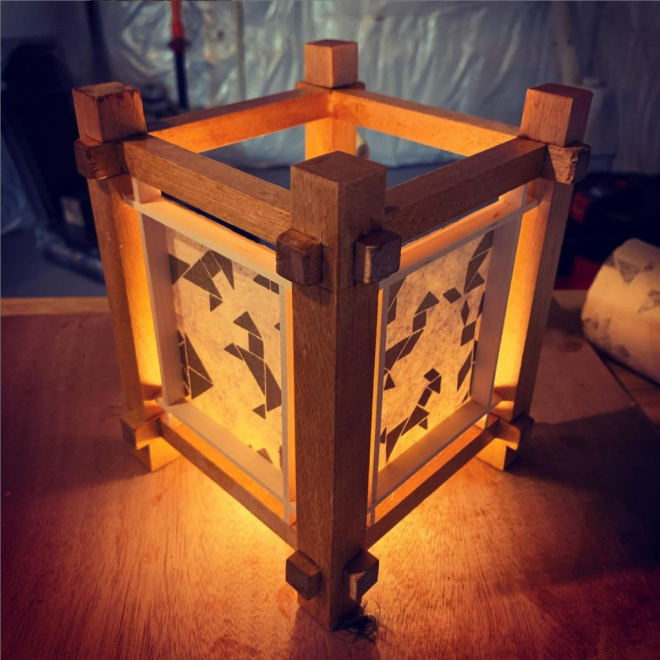
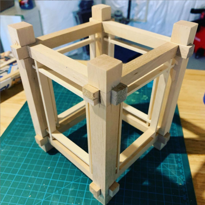
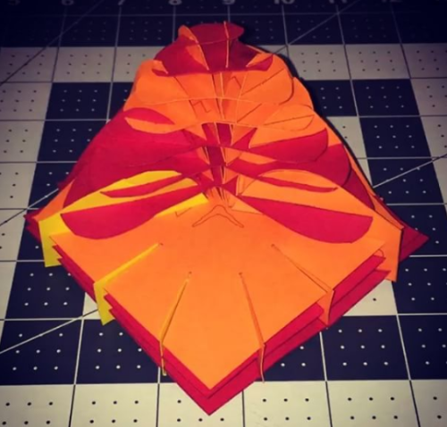
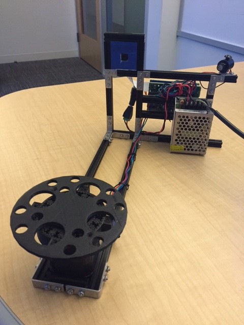
The complete setup should look like this:
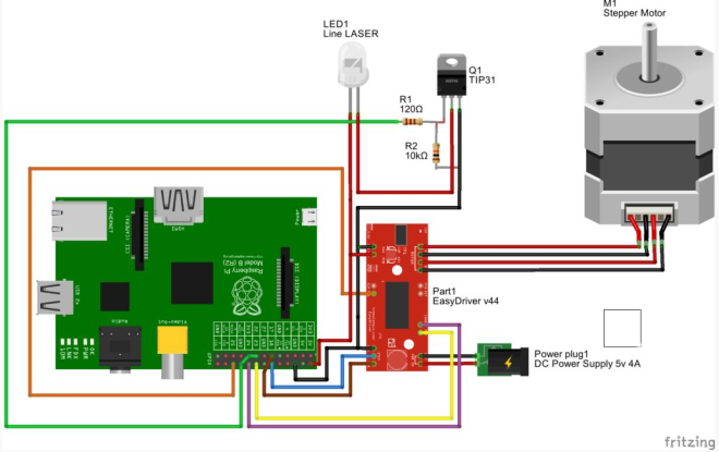
Task 2: Preparing the hardware circuits
I have used the Raspberry Pi Rev B board for this project. I am also assuming that the Pi Camera is connected to the camera port on the board. The circuit diagram assumes the pin layouts match this board.
There are two main parts to the hardware setup:
- Stepper motor control
- LASER switch control
Stepper Motor Control
For the Stepper motor control circuit, we are using the EasyDriver board (link). This board takes away all the pains of having to build a voltage-regulated power supply that can deliver consistent and enough current to run a stepper motor, along with the PWM control signals required to run them. With this board, all we need to do is connect a dc power supply with a high-enough current rating (4 Amps is sufficient), connect the control lines to IO pins on the Raspberry Pi, connect the stepper motor to the motor output, and you are ready to go! It really is that simple. Thanks Brian!!!
And Did I mention that EasyDriver also provides a regulated 5v output that can drive other circuits? Well, yes it does! So we will be powering up the Raspberry Pi and the LASER diode with this regulated supply! Double Thanks Brian!!!
The EasyDriver requires the following inputs:
- ENABLE– When this control signal is low (0v), the motor output is enabled and what signals are applied to the other control signals, get propagated to the stepper motor. We connect this pin to one of the IO pins on the Raspberry Pi (Pin 24). We have to remember to set this pin to logical 0 whenever we want to enable the stepper motor and to logical 1 whenever we want to disable it.
- MS1and MS2 – These two control signals control the micro-stepping mode of the stepper motor. The stepper motor usually takes about 200 steps to complete one full rotation – with a step-size of 1.8 degrees. Micro-stepping allows you to break this into smaller steps – 1/2, 1/4, or 1/8. Essentially this means that it allows you to reduce the step-size to 0.9, 0.45 or 0.225 degrees respectively, allowing finer control on the rotation. We connect MS1 to Pin 25 and MS2 to Pin 23 on the Pi. Setting the pins to (0,0) tells the driver to run the motor without any micro-stepping. Setting the pins to (1,1) tells the driver to run the motor with the smallest step-size – 1/8th. The values in between are left to you to decipher.
- STEP– this control line drives the stepper motor. When we apply a pulse to this line (000011110000), the driver moves the stepper motor by one step when the line transitions from 1 to 0 (also called the falling edge of the pulse). We connect this line to Pin 18 of the Pi. We will write a small MATLAB function to send a pulse on this IO pin. More about that in the software setup.
- DIR– this control line decides whether the stepper motor will rotate in the clockwise or counter-clockwise direction. We will connect this line to Pin 17 of the Pi. Setting this line to logical 0 makes the stepper rotate in clockwise direction and logical 1 makes it rotate in the counter-clockwise direction.
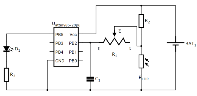
LASER Switch Control
For the scanning setup, we need a mechanism to switch the LASER diode on and off when required. We accomplish this using a very simple transistor switch circuit. We use a NPN transistor (TIP31) in the common-emitter configuration and a voltage-divider bias (Wikipedia). In our circuit, R1 is the 120-ohm resistance and R2 is the 10 KOhm resistance. Pin 22 of the Pi is connected to the outer lead of R1. When we set this pin to logical 1, it is equivalent of tying R1 to Vcc. By ensuring that voltage across the base and emitter is higher than the forward bias, we allow the current to flow through the collector and thereby activating the LASER diode. When we set this pin to logical 0, it is equivalent of typing R1 to ground, pulling the voltage across the base and emitter to zero, switching off the current through the collector and deactivating the LASER diode.
The LASER diode has two leads – power and ground. The power lead is connected to the +5v supply coming from the EasyDriver and the ground lead is connected to the collector of the NPN transistor.
Note: It is important to tie the ground of the +5v supply from the EasyDriver and the ground of the Raspberry Pi together to ensure the control signals coming from the Pi have a common ground.
I would recommend that you test the entire circuit on a breadboard before assembling it on top of the prototyping shield so that there is no need for any costly reworks!
Task 3: Getting the Software together
For the software, we need to do two things:
- Prepare the Raspberry Pi to communicate with MATLAB using the hardware support package. You can get the details about that here:
http://www.mathworks.com/help/supportpkg/raspberrypiio/functionlist.html
- Once you have setup the SDC and plugged it into the Raspberry Pi, you need to open the Rasp3DScanner project in the MATLAB guide interface. This is a simple GUI interface for the scanner. Make sure that you have changed the current directory to point to the folder containing the scanner code you downloaded from MATLAB File Exchange.
Code Walkthrough
You should see the following files in the Rasp3DScanner archive:
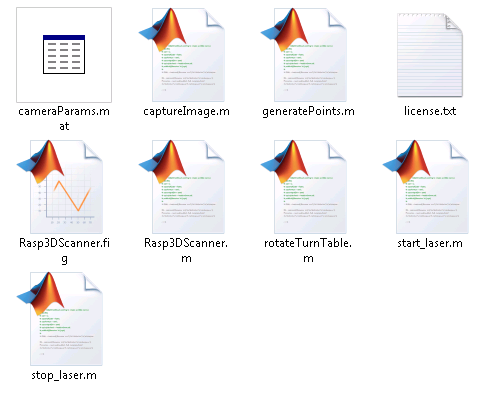
Rasp3DScanner.fig is the main GUI file and can be launched from MATLAB console by typing “guide” and selecting the Rasp3DScanner project from the browse field. Rasp3DScanner.m contains all the code for the application and implements the scanning algorithm. There basic utility functions that are self-explanatory in the sense that they control the functioning of the LASER, the Stepper motor and camera.
The cameraParams.mat file contains calibration data from my setup. You should regenerate the cameraParams.mat file for your setup by following the steps here:
http://www.mathworks.com/help/vision/ug/single-camera-calibrator-app.html